A fast moving source of light on a sufficiently long exposure photograph will look like a bright continuous streak (think of photos of fire dancers). Similarly, a sufficiently fast moving light source would look like a long streak to our eyes too, which permits a number of interesting persistence of vision Arduino projects where carefully timed light sources create the illusion of images floating in space.
One can use this effect to make a projector where a fast moving laser dot traces out a vector image on a wall. Two mirrors mounted on angular actuators would direct the laser light along a path in the xy plane tracing the same image tens of times per second.
The laser
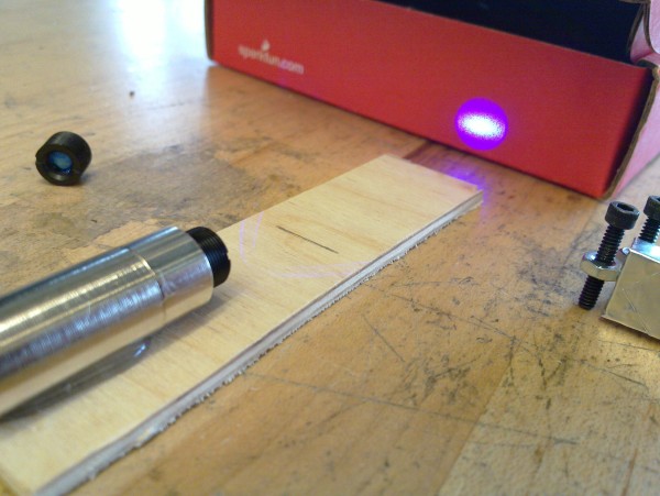
Let’s start with the laser. You can buy cheap laser modules of a great variety of colors online. For this build I chose purple.
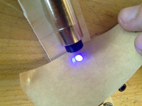
As you can see in the image above, the beam from the laser is not circular (it is not Gaussian). The next image confirms it and shows some higher-order bright circles as well:
Due to diffraction that type of beam will diverge significantly. Instead, I want a nice circular beam (Gaussian beam) that diverges little over multiple meters. This can be done with a spatial filter:
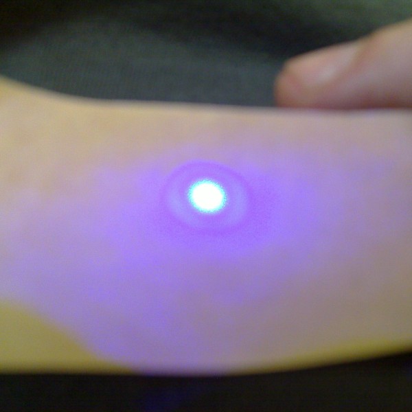
In my case this is just a small tin-foil diaphragm on which the laser is focused, hence creating a “perfect” point source and a convergent lens after the diaphragm to create a parallel beam (for those interested, the waist of the beam was set to a few meters downstream from the filter). Here is the resulting filtered beam - nicely circular with a pretty Airy disk.
Steering the laser dot
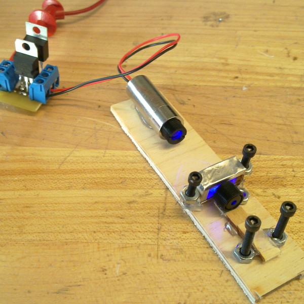
Now it is time to attach the mirrors that will be steering the beam. Their rotation axes will be at 90 degrees, so that one of the mirrors controls the x coordinate of the point while the second mirror controls the y coordinate.
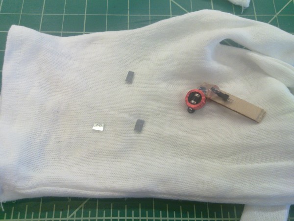
The mirrors are mounted on small magnetic coils (actuators from an RC plane). By controlling the current in the coils we can control the displacement of the mirrors and hence the position of the laser dot.
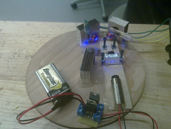
And here we have everything together (excluding the small sound amplifier that drives the mirror coils). The entire thing is driven by the headphones output of my laptop (or if you generate the waveform in advance you can just put it on a small mp3 player).
This already works great for generating circles and Lissajous
curves - just generate
sine waves of the corresponding frequencies and amplitudes. If you want a
rotating Lissajous figure as below, just add a small detuning between the x and
y frequency. You can use sox under Linux and other OSes to generate the wave files.
The dot slowly moving on a circle:
The dot tracing out a fast slightly-detuned Lissajous figure:
Some Math
An issue arises at this point. The actuators on which we mounted the mirrors have their own resonant frequency. Driving them with an electric signal at that frequency will produce very different results from driving them at some other frequency. This is not a problem if we want to produce simple Lissajous figures, but for more complicated images our signal will carry components of many different frequencies. For instance we want to draw five-petal flower: the signal will have two main components - a sine wave at the frequency at which we are redrawing the image (this alone will draw a circle) and on top of this we will add a sine wave at 5 times that frequency (for drawing the petals). We will employ two mathematical tools to address this issue: Fourier transforms for decomposing the image in its sine wave components and transfer functions of harmonic oscillators for modeling how the mechanical actuators respond to that electric signal.
You can skip the math and go straight for the plots.
The Response Function of The Mirrors
We will measure the displacement that the mirrors produce for different electrical signal. From this we will deduce their spectrum (or transfer function).
For the x and y mirrors we have (assuming perfectly perpendicular mirrors for the moment):
\({\frac {{\mathrm {d}}^{2}x}{{\mathrm {d}}t^{2}}}+2\zeta_x \omega _{0x}{\frac {{\mathrm {d}}x}{{\mathrm {d}}t}}+\omega _{0x}^{2}x=\xi\) - green wire
\({\frac {{\mathrm {d}}^{2}y}{{\mathrm {d}}t^{2}}}+2\zeta_y \omega _{0y}{\frac {{\mathrm {d}}y}{{\mathrm {d}}t}}+\omega _{0y}^{2}y=\upsilon\) - yellow wire
- \(x,\, y\) are the deviations of the laser beam position in arbitrary units (x is the green wire, y is the yellow wire)
- \(\zeta,\, \omega_0,\, f_0\) are the damping coefficients, angular and ordinary resonant frequencies
- \(\xi,\, \upsilon\) is the input signal in mV
In the Fourier domain (ordinary frequency):
\((2\pi i f)^{2}{\hat {x}} + 2 \zeta_x \omega_{0x} (2\pi i f){\hat {x}} +\omega_{0x}^{2}\hat{x}=\hat{\xi}\) and similar for y
i.e.
\(Y_x(f) = (2\pi i f)^{2} + 2 \zeta_x \omega_{0x} (2\pi i f) +\omega_{0x}^{2}=\frac{\hat{\xi}}{\hat{x}}\) and similar for y
rewriting in only ordinary frequencies
\(Y_x(f) = (2\pi)^2\left(2 i \zeta_x f_{0x}f +f_{0x}^2-f^2\right)=\frac{\hat{\xi}}{\hat{x}}\) and similar for y
Finding \(\zeta\) and \(f_0\) (and introducing scaling) from the spectrum
We are measuring the amplitude of the response to a sine drive:
\(|Y_x(f)|=scale_x (2\pi)^2\left|2 i \zeta_x f_{0x}f +f_{0x}^2-f^2\right| = \left|\frac{\hat{\xi}}{\hat{x}}\right|\) and similar for y
and fitting \(\zeta\) and \(f_0\) and \(scale\).
We introduced \(scale\) because given that we are measuring the displacement in arbitrary units we have one more degree of freedom. For engineering reasons we also have to limit this displacement to 5 units (after that nonlinear effects might appear).
We could also measure \(scale\) at the DC regime if we are so inclined.
Note: The measurements below were done by hand for preliminary testing purposes. As they were not precise enough I performed more precise automated measurements and redid the protocol described here (discussed below).
However the mirrors are not perfectly perpendicular
The real deviations are
\(x^\prime \approx x + \frac{3}{8}y\)
\(y^\prime \approx y\)
But like above we would like a generic parametrization so we will write it as
where
.
The \(M\) coefficients were deduced from the same set of measurements as above, but a more precise measurement might be necessary at some point. The diagonal of M has to be only ones, otherwise it will be degenerate with the \(scale\) variables.
The complete pipeline (assuming infinite electrical power)
Assuming infinite power for the electrical signal! This makes the math easier - very sharp turns in the path of the dot require great spikes of voltage to make the mirrors switch directions fast enough. We will see below what happens when we acknowledge that such spikes are impossible.
Working in Fourier space:
and in reverse:
Putting the math in practice
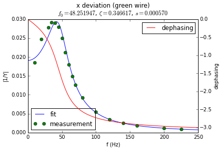
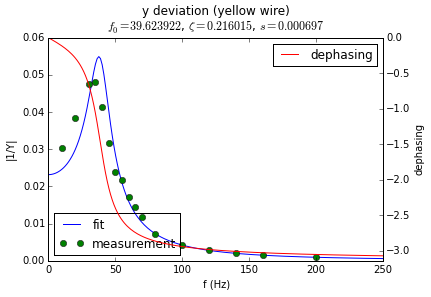
Below are the spectra of the two mirrors. The vertical axis represents the displacement that the mirror produces for an electrical signal of fixed amplitude and of frequency represented on the horizontal axis. The green dots are measurements I took by hand with a ruler for electric signals generated by my computer’s sound card.
As you can see both mirrors have their resonance at around 30 to 50 Hz. At higher frequencies their response quickly becomes very small.
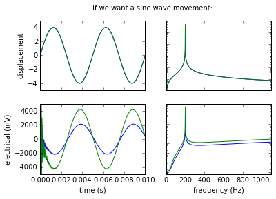
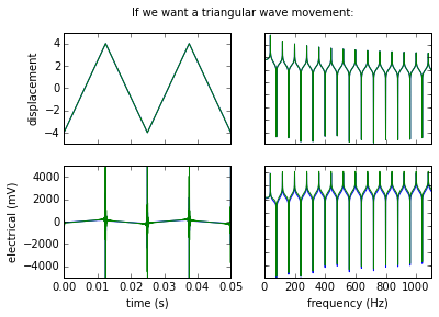
In the following set of plots I compare the electrical signal (lower half) with the displacement that signal would produce in the mirrors (upper half). The left side represent how the signal and displacement look in the time domain. The right half represents the signals in the frequency domain (i.e. it is the Fourier transforms).
Here we want to produce sine displacement in both mirrors with the same amplitude. Given that the two resonant frequencies are different, the required electric signals are slightly different and slightly dephased from one-another.
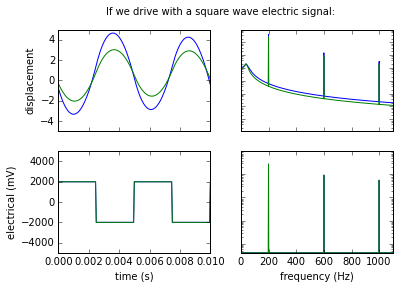
Here we see that simply driving with a square wave does not produce square displacements (the higher harmonics in the square wave get filtered out).
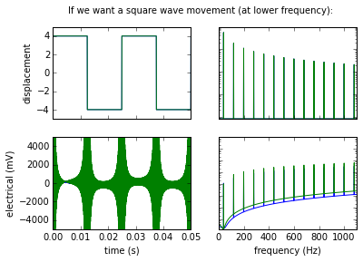
But if we set the target to be a square displacement we can calculate the necessary electric signal. As you can see, the required signal is quite crazy:
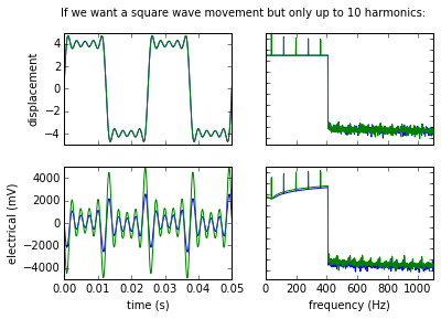
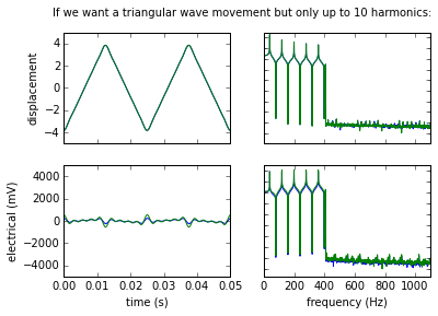
By filtering the higher harmonics at a more reasonable cutoff frequency we can obtain something that approximates a square wave with a not too crazy electric signal that we can actually generate:
And here we do the same for a triangular displacement (we can see slight rounding of the edges when we apply the high-frequency filter).
Getting a more precise spectrum
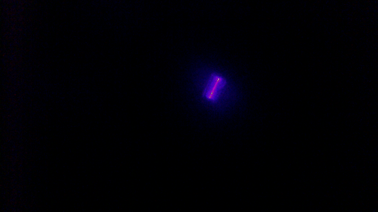
Doing the displacement measurements by hand was not particularly fun. It would take too much work to get enough data points by hand to produce a precise spectrum. For that reason I wrote a small script that generates sound waves of different frequencies and fed the headphones’ output to the actuators. At the same time the webcam of my computer was taking pictures of the ceiling where the laser dot was projected. With enough such pictures I was able to get much more precise reconstruction of the spectrum of the actuators.
for FREQ in {20..100}
do
    echo $FREQ
    play -n synth 3600 sin $FREQ remix 0 1 2>/dev/null &
    PID=$!
    sleep 2
    cvlc -I dummy v4l2:///dev/video0 --video-filter scene --no-audio --scene-path . --scene-prefix ${FREQ}_01_ --scene-format png vlc://quit --run-time=20 2>/dev/null
    kill -TERM ${PID} 2> /dev/null
    play -n synth 3600 sin $FREQ remix 1 0 2>/dev/null &
    PID=$!
    sleep 2
    cvlc -I dummy v4l2:///dev/video0 --video-filter scene --no-audio --scene-path . --scene-prefix ${FREQ}_10_ --scene-format png vlc://quit --run-time=20 2>/dev/null
    kill -TERM ${PID} 2> /dev/null
done
It takes images like this:
And with some simple use of numpy arrays (no fancy image processing libraries) I measure the size and angle of the streak in the photo:
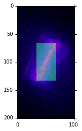
After an hour of data acquisition and a minute of data processing I get a much more detailed reproduction of the spectrum:
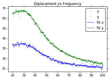
Which can finally be used for generating more complicated images.
Here is a test video. It starts with a small expanding rotating star, then it goes to a dancing circle, then to a dancing square and then back to a dancing star.
There is still more calibration to be done, but as a proof of concept I am quite happy with this prototype.
The code used for the data processing, including all the spectrum analysis, signal synthesis, and computer vision is available here.