My current institution, the Yale Quantum Institute, a leading research center on quantum computing, has had an Artist in Residence program for the last year, initiated by our manager Dr. Florian Carle. During the year Martha Lewis has been part of the institute, setting up multiple exhibits and working with the researchers at the instute through numerous art workshops.
You can read more about Martha’s work at YQI on the YQI website.
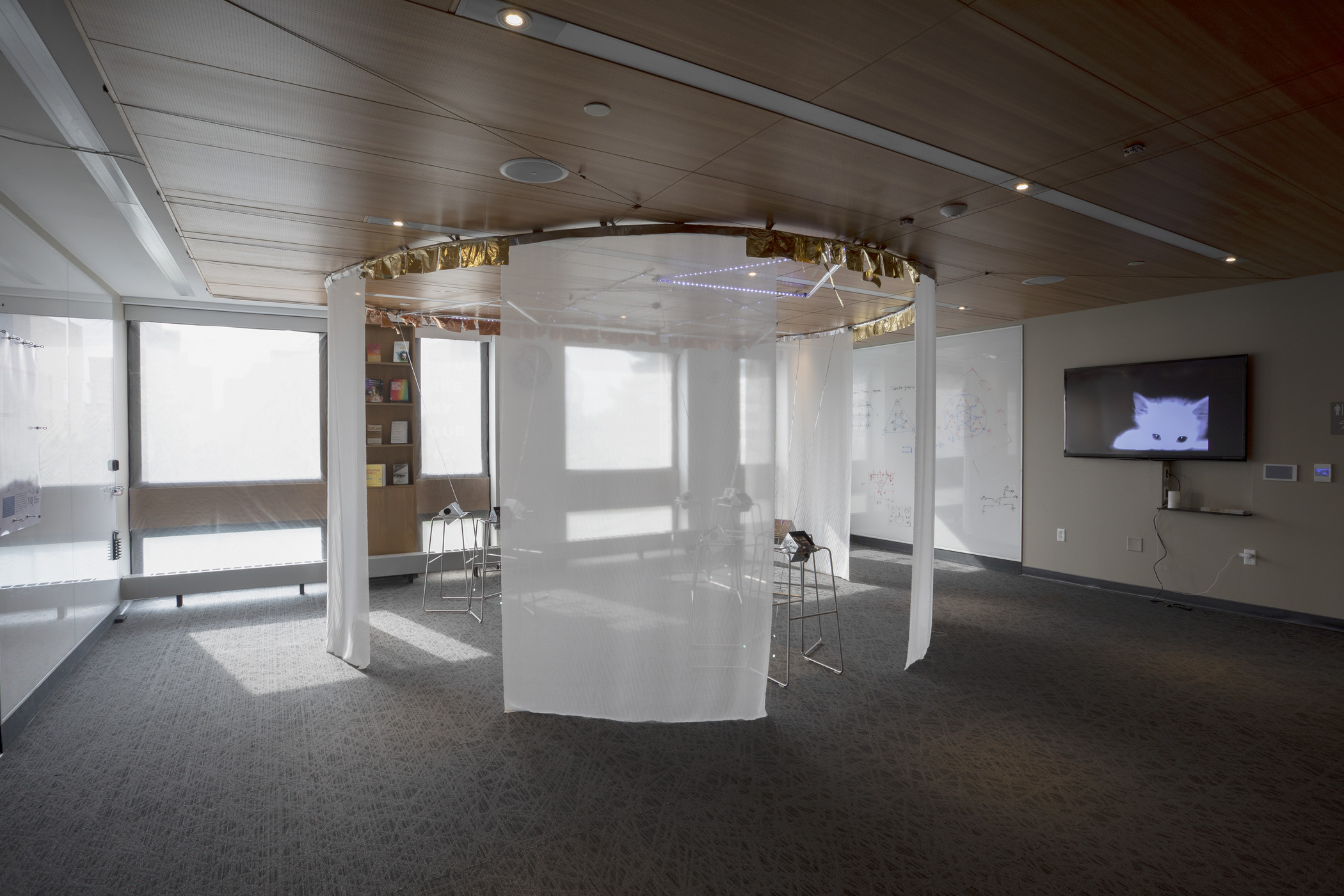
For the end of her residence, Martha prepared an amazing interactive installation, on temporary exhibit in the main hall of the institute, where each visitor gets to experience (and interpret for themselves) many of the counter-intuitive properties of quantum mechanics.
More about the artwork can be found at YQI’s website, however, I would like to discuss a particular part of the installation. The ceiling diagram, suggested by Prof. Devoret, is a graph represantation of a subset of the Pauli group of two qubits, that can be used to clearly illustrate the trouble one faces when trying to explain quantum mechanics while using only classical macroscopical intuition. Below, I will describe both the physical principles on exhibit, and the embedded electronic contraptions that permitted the installation to interactively respond to the guests.
If you are specifically interested in how to set up a Raspberry Pi or a similar microcontroller to perform motion sensing (and transform the sensed motion into some form of a visualization) skip the next section.
Non-contextual Hidden Variable Theories
On exhibit in the installation was the spooky counter-intuitive behavior of the quantum world, and in particular, the failure of classical intuition when dealing with it.
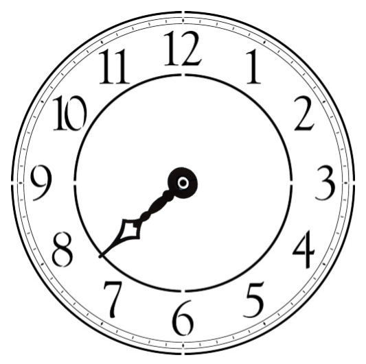
Chief among the failures of classical physics in explaining the quantum world, is the expectation that all observable quantities have a definite (but maybe not yet known) value, even before they are observed. For instance, imagine an arrow (the hour arrow on a clock face for instance). The arrow can point mostly upwards (9 to 3 o’clock) or mostly downwards (3 to 9 o’clock). At the same time the arrow can point mostly to the left (6 o’clock to 12 o’clock) or to the right (0 o’clock to 6 o’clock). We can measure the arrow’s orientation both in the vertical and in the horizontal direction. For instance, 2 o’clock corresponds to an arrow that is both upward and rightward oriented.
| Up/Down Orientation | Left/Right Orientation | |
|---|---|---|
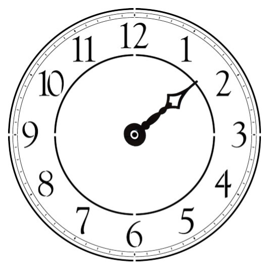 | ↑ | → |
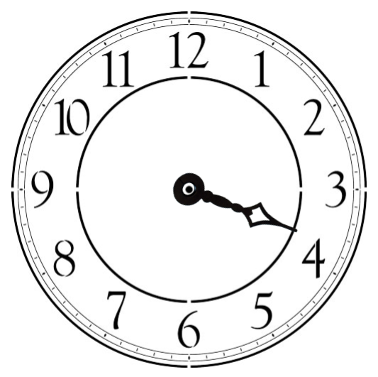 | ↓ | → |
 | ↓ | ← |
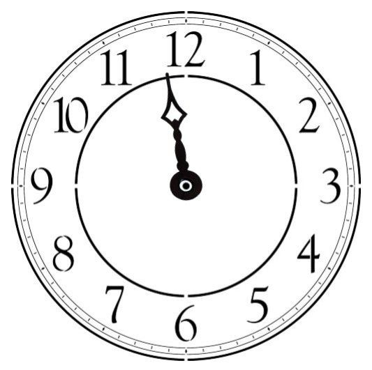 | ↑ | ← |
This idea is so natural that nobody ever thinks to even put it in words: an arrow has a definite orientation along both the horizontal and the vertical direction. Even if you put the clock face in a closed box and do not observe the inside of the box, the arrow would still have a definite orientation (up/down, left/right). Any two observables in the macroscopical world are compatible and can be measured together, whether it is the horizontal/vertical orientation of an arrow, or the velocity/position of a particle.
However, this notion of compatibility between observables (the term of art is commutativity, i.e. the two observables commute if they can be measured consistently together) breaks down if you try to observed small, cold, and well isolated entities (like the velocity and position of an elementary particle, or the horizontal/vertical orientation of the axis of rotation of an electron). In particular, the impossibility of measuring both velocity and position precisely is known as Heisenberg’s uncertainty principle.
| Hilbert space vector | Up/Down Orientation $$\sigma_z$$ | Left/Right Orientation $$\sigma_x$$ | |
|---|---|---|---|
 | $$\begin{pmatrix}+1 \\ +1\end{pmatrix}$$ | ? | → |
| $$\begin{pmatrix}+1 \\ 0\end{pmatrix}$$ | ↓ | ? |
| $$\begin{pmatrix}+1 \\ -1\end{pmatrix}$$ | ? | ← |
| $$\begin{pmatrix}0 \\ +1\end{pmatrix}$$ | ↑ | ? |
The “Hilbert space vector” column is for reference for those with the background, but it is not important for our discussion. Spin cartoon by Tanedo
In our example with the arrow, we can consider a very small arrow, like the direction defined by the axis of rotation of an electron. This arrow (the term of art is spin-\(\frac{1}{2}\) particle) can be measured in the horizontal direction (to learn whether it points left or right) and in the vertical direction (to learn whether it points up or down). If we measure the horizontal orientation twice, we will get the same result the first and the second time. This is not too surprising: it would be a pretty lousy measurement, if our measurement causes the measured entity to flip. A major goal of experimental science is to find ways to noninvasively measure the world without affecting and changing the target of the measurement. However, this is exactly one of the surprises that quantum mechanics brings to the table: nobody, not even an angel, can measure the horizontal orientation of our quantum arrow without destroying the information we had about the vertical orientation of the arrow. If we measure the horizontal orientation, then the vertical one, then the horizontal again, the first and the last measurement will be the same only half of the time, because the other measurement done between them perturbed the system.
| 1. Initial unmeasured state (possibly a superposition) | 2. Measure the Left/Right orientation | 3. We happen to get a “right facing” electron | 4. Measure the Up/Down orientation | 5. We happen to get an “up facing” electron | 6. Measure the Left/Right orientation again | 7. We happen to get a “left facing” electron, without a trace that the electron used to face right after the first measurement. |
|---|---|---|---|---|---|---|
|
We will “project” the electron in a “left” or “right” state. | |
We get either up or down facing electron with probability 1/2. | |
Indipendentaly of the previous state we get either left or right facing electron with probability 1/2, completely unaware of the orientation reported at the first measurement. | |
The existence of such incompatible (non-commuting) observables is one of the first surprises of quantum mechanics. It has spread to popular culture as the Heisenberg uncertainty principle (that only velocity or position can be precisely measured, but never the two at the same time), but as we have seen, it applies to many other observables.
We used an example about the orientation of a quantum arrow (spin-\(\frac{1}{2}\) particle) instead of the more well understood velocity/position example, because this system enables us to discuss another, far more wondrous, feature of quantum mechanics, sometimes named contextuality. We will try to give a taste of its weirdness below.
It is not too difficult to explain the non-commutativity of quantum observables (or more generally, the observer effect) by saying that when the system we try to measure is small, even the finest of measurements will slightly perturb it. As such, the uncertainty principle, whether about the orientation of an arrow or the position and velocity of a particle, does seem peculiar, but hardly counterintuitive. We can just say that in the sequence of horizontal, vertical, and a second horizontal measurement, the vertical measurement is simply always too rough, and it might cause a flip on the horizontal direction which becomes noticeable in the second horizontal measurement.
However, a hundred years of both mathematical constructs searching for contradictions and progressively more refined experiments have shown that this is not the whole truth. The incompatible vertical measurement did not simply perturb the system, rather it erased the notion of a horizontal orientation for our arrow. Before the repeated horizontal measurement, our arrow did not have a hidden unknown horizontal orientation. Instead, it “decided” what horizontal orientation to have the moment we measured it (and it also stopped having a defined vertical orientation).
The notion that the arrow has both definite vertical and definite horizontal orientation (even if one of them happens to be unknown at the time because the last measurement jiggled it in an unpredictable fashion) is called a hidden variable theory. And that notion, as intuitive as it sounds, is completely refuted by simple thought experiments in which one tries to assign definite values to all possible observables of a system: If one tries such a thing, they inevitably are led to a contradiction where one of the observables needs to have two values at the same time. The only way to break through this contradiction is to dispense with the notion of definite (but unknown) values of the observables. If we have not measured something, its value is not simply unknown, it is undefined.
In particular, the ceiling diagram of the art installation, showcases what would happen if one tries to consistently give definite values to the relative orientation of two quantum arrows. One will always be left with a requirement that the arrows at the same time point in the same and in the opposite direction - an obvious contradiction.
While absurd on first sight, embracing the idea that observables do not have definite (but maybe unknown) values until they are measured, dispenses with the above contradiction. And it further has proved itself in the last century, by enabling us to predict the quantum phenomena that power our civilization’s technology.
For a more detailed, but fairly dense discussion of this notion of contextuality you can consider this poster and the references within. A lighter and easier to read version of it would have to wait for next time (the PDF is added as an inset below, but on Firefox it renders poorly if it renders at all).
The electronics enabling the art installation
To visualize this wondrous but counter-intuitive quantum behavior, we put an interactive version of the diagram inside the installation. The diagram represents the state of two qubits. Each triangle on the diagram represents a set of consistent (commuting) measurements you can perform on the simulated quantum system and the colors on the vertices of each triangle represent the value of the given measurement (blue for +1 and red for -1). At any given point, only one of the triangles can be “measured” - if another triangle is measured after that, information from the previous triangle is lost.
The interactive part of the diagram comes from the fact that the decision of which triangle is to be measured comes from the location of the visitor: a fish-eye camera placed on the ceiling detects motion, and depending on in which location the motion was observed, the corresponding triangle would be set as the active one.
The Raspberry Pi picamera library provides a great foundation on which to
build the motion detection. First we create a low-pass filter that measures
(and filters) the total displacement observed at each pixel block in view:
class LowPassDetectMotion(picamera.array.PiMotionAnalysis):
    '''The motion detection routine.'''
    filtered = None
    def analyze(self, a):
        now = time.time()

        # Image acqisition and filtering

        # set the "decay" in the filter, where `TAU_IMAGE` is the characteristic decay time
        beta = math.exp(-(now-global_lasttime)/TAU_IMAGE)
        alpha = 1-beta
        # get the current total displacement per pixel block from the camera (x_displacement**2+y_displacement**2)
        a = np.sqrt(a['x'].astype(float)**2+a['y'].astype(float)**2)
        # perform the filtering operation (a weighted average of the old and the new value)
        if self.filtered is not None:
            a = alpha*self.filtered + beta*a
        self.filtered = a

        # Find the most active location in the image

        # coarse grain the image into a 4-by-5 grid
        grid = a.reshape(4,H//4,5,W//5).sum(axis=(1,3))
        motion = np.max(grid)

        # find where in that grid we have the larged amount of motion
        h,w = [int(_) for _ in  np.unravel_index(np.argmax(grid), grid.shape)]

        # `h` and `w` can be assigned to some global variables or singleton objects
        # in order to be used by other parts of the software
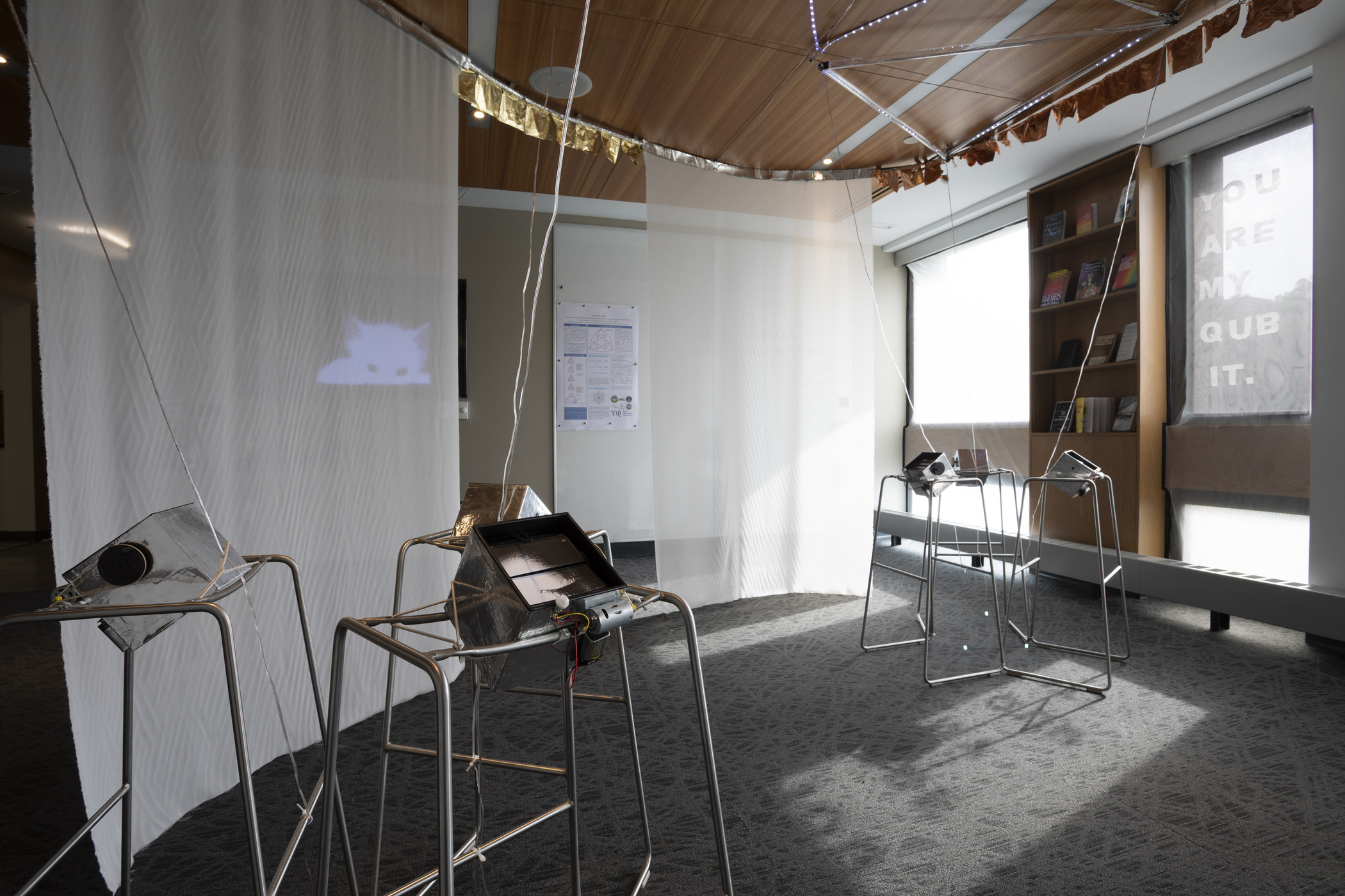
The rest of the script running on the microcontroller can be found here. For the LEDs, we used the common and cheap hobbyist favorites ws2812b LED drivers. A couple of independent low-power motion sensing LED “blinkies” were spread around the institute building. A number of motion sensing flip books with imagery tailored to the exhibit by Martha was arranged below the diagram.
Some visuals
Here is the ceiling diagram inside of the larger art piece (meant to resemble the large cylindric cryofridges in which typical quantum information experiments take place). Each part of the exhibit, from the silk drapes to the mechanized flipbooks is meant to react and be perturbed by the observers of the installation.

You can see Martha walking through the installation she designed, while the ceiling diagram responds to her motion, keeping the colors consistent with the constraints imposed by the Pauli group of two qubits.
In parallel with the motion sensing, we ran image acquisition, which enabled some rather pleasant timelapses (without filtering out the infra-red component of the image). Adorably, one can see the flipbooks rotate as people move past them.
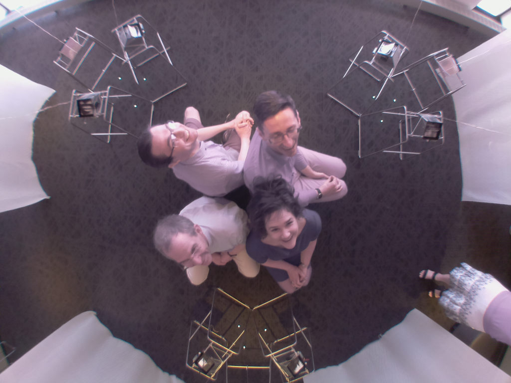
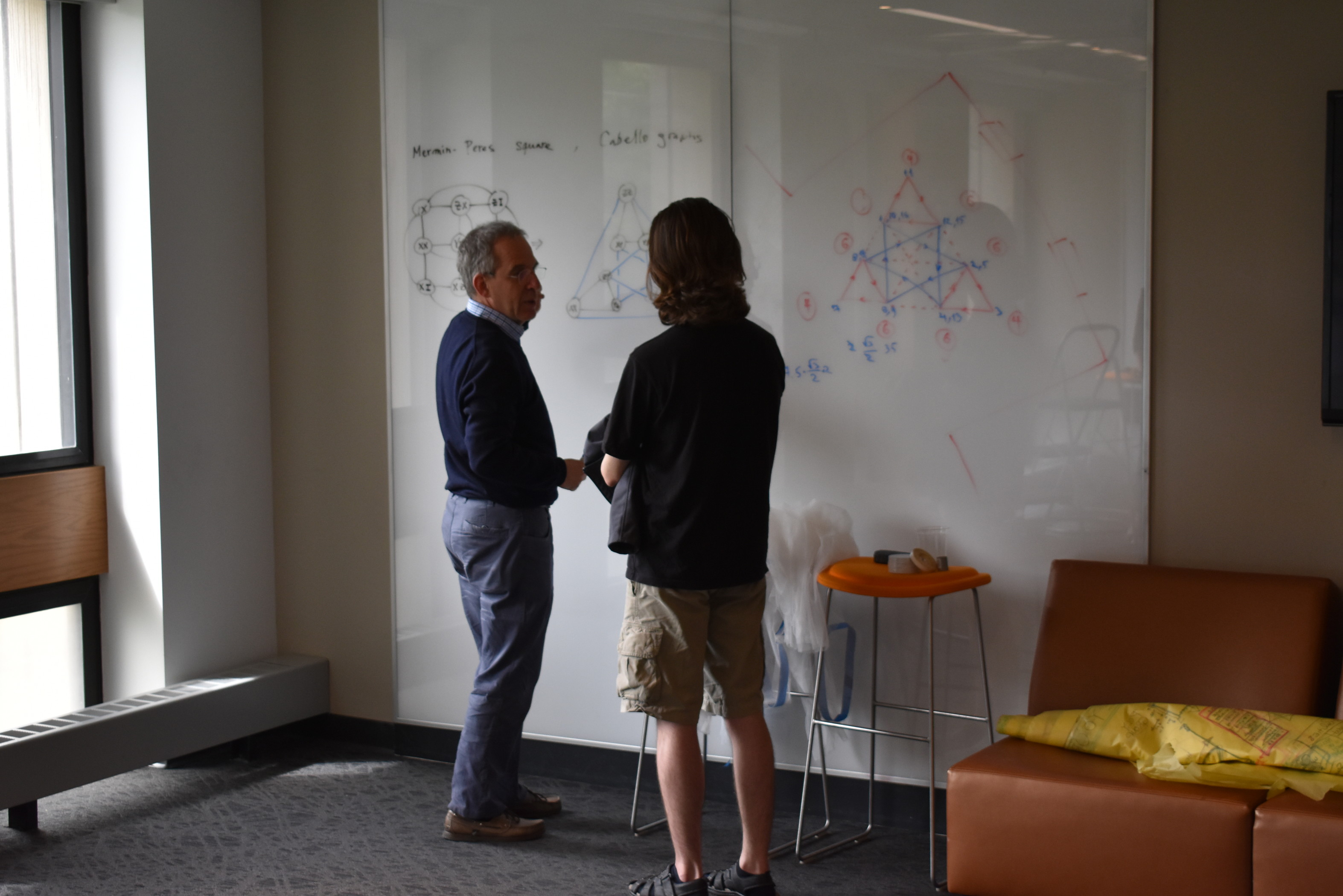
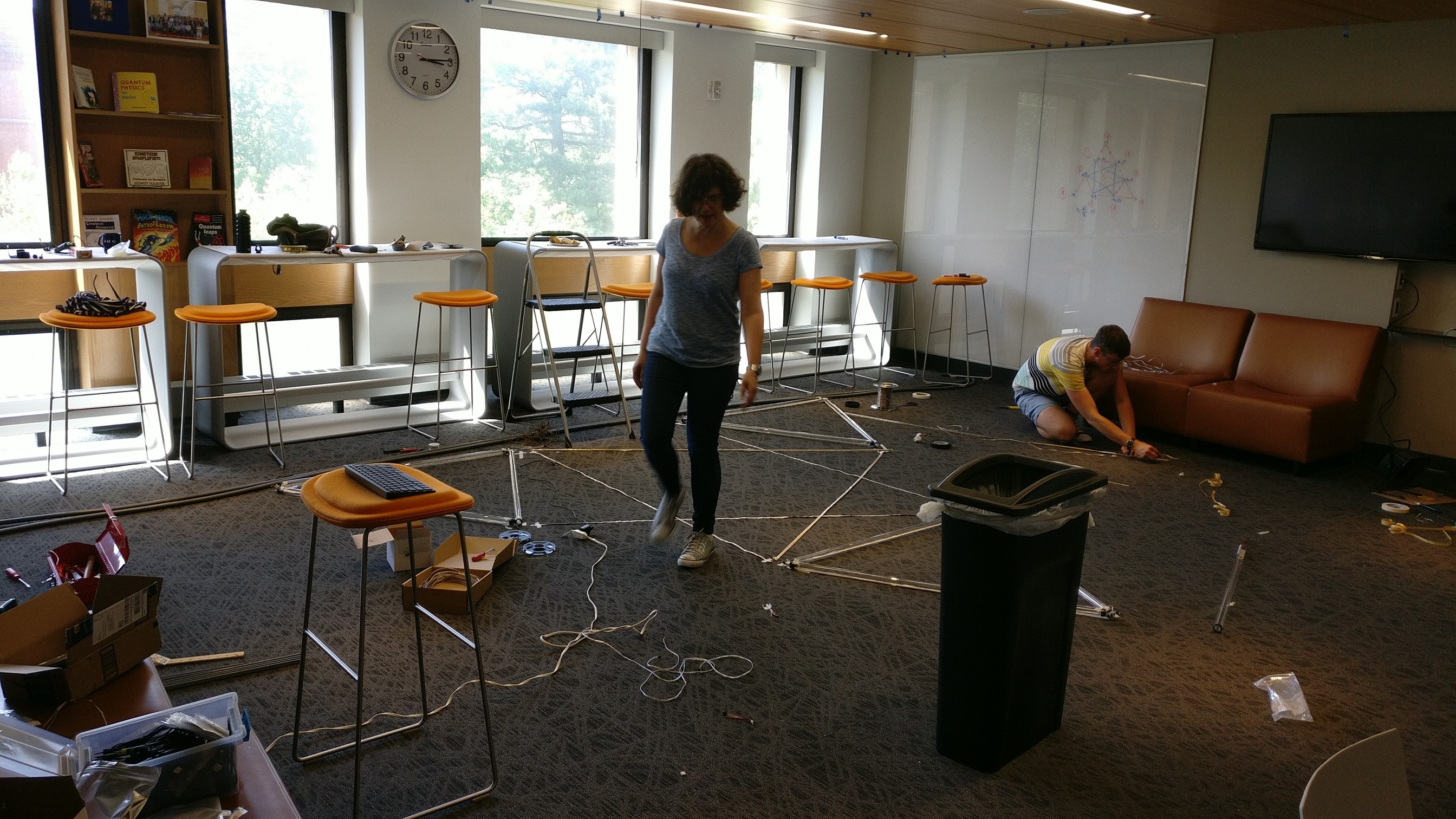
And a picture of the people involved in the project (Martha Lewis, Dr. Florian Carle, Prof. Michel Devoret, and me) and some prep work: